Dammit Jim!

I end up generating a lot of postscript plots in R and other programs. Unfortunately, a lot of not so technical people have trouble opening postscript files so I end up having to convert these images to other formats pretty often. A really handy program for converting eps files to png (or jpg although that’s not really an optimal format for plots) is ImageMagick (available for all OSs I believe). ImageMagick lets you quickly convert (and create thumbnails, make B&W,…) from the command line without having to open up Photoshop.

For example, to convert an image named myPlot.eps to png you just need to enter convert myPlot.eps myPlot.png (convert is a program in the ImageMagick package) at the command prompt and you’ll get a png file in myPlot.png. If you want to adjust the resolution (the default resolution is 72 dpi) of the output image, you can add the -density option (e.g. for 200 dpi convert -density 200 myPlot.eps myPlot.png). Make sure you put the -density part before the input image name.

Converting many files at once is where ImageMagick really shines. The mogrify command is probably the quickest option. For example, to convert the files image01.eps, image02.eps and image03.eps to png, just use the command mogrify -format png image*.eps. In one shot, it will create image01.png, image02.png and image03.png.

Unfortunately, recent version of Imagemagick seem to be treating eps to png conversions oddly (see below) so mogrify isn’t cutting it on my files. If you have similar trouble (and you’re on Unix or Mac or Cygwin), you can just use a bit of Bash combined with the convert command to get around the problem like this:

[bash] for f in `ls *.eps`; do convert -density 100 $f -flatten ${f%.*}.png; done [/bash]

Black Background Problem

As I mentioned above, I started having trouble converting from eps to png after upgrading to ImageMagick 6.4. The transparent/white backgrounds in my eps files were being converted to black backgrounds and making the figures unreadable. I guess it must be some change in how transparency is handled but I’m not totally sure what changed. It took me a bit of googling before I found the solution, so I’ll repost it here. Adding -flatten to the command (e.g. convert myImage.eps -flatten myImage.png) should change the background back to white. My mogrify command doesn’t include the -flatten option so convert (like the example above) seems like the way to go.

We just picked up a little Acer Aspire One netbook. We’re pretty happy with it so far (except we’ll be exchanging it for a new one since the ‘p’ key on this one only works half the time). I’ll probably do a more in depth review once we’ve used it a bit but it certainly is tiny and handy. The only major drawback is the tiny mousepad. Anyway, it doesn’t come with a system restore or Windows disk. I realize there’s a hidden partition on the hard drive but I don’t really like trusting a single hard drive. Google didn’t turn up any really handy answers for how to make a system restore disk from a hidden partition or an entire install (especially onto a USB hard drive) using free software so I thought I’d document what I ended up coming with. I have no idea if this is the smartest/safest way to do this and I’d recommend getting Norton Ghost or something similar if you don’t feel confident with any of the processes in here.

There’s two steps to the process, making a USB drive into a little bootable linux system and backing up the partitions onto a USB hard drive.

Things You’ll Need

• Some annoying computer with no backup/restore CD
• USB Key Disk
• USB Harddrive

I think you could actually just do this with a single harddrive or a really big USB key if you made it into 2 partitions (the SystemRescueCD OS doesn’t save changes by default).

Making a bootable linux USB disk

I used SystemRescueCD for my linux system (although I suppose any small distribution with the appropriate tools would work). Obviously a CD does not do a lot of good when you have a laptop without a CD player but luckily (the somewhat misnamed) SystemRescueCD can be installed to a USB drive. As documented on that page, you’ll need to download the .iso from the SystemRescueCD site and move most of the files from the .iso to your USB drive. If you don’t already have a handy way to mount an .iso and don’t feel like burning a CD, I had decent luck with Microsoft Virtual CD-ROM Control Panel or if you’re using Linux just a simple mount -o loop disk.iso /some/empty/folder (although for some strange reason I had trouble getting a Linux-made version working). Once you’ve copied the files from the CD and ran syslinux as directed, you should have a handy USB key that will boot a computer into linux (if you set the BIOS to boot from USB).

Backing Up Partitions

Once you’ve got your little USB linux, you’ll want to look at Lifehacker’s handy walkthrough to SystemRescueCD. Replace all mentions of CD with USB disk and instead of backing up to the same hard drive, we’ll back up to an additional USB hard drive.

Now from here on out, you’ll want to be very careful. Things should be (mostly) safe but messing around with partitions is getting towards the more touchy end of computing. I’d back up anything important to a separate harddrive. After that, here we go:

1. Turn off your computer, stick in your USB key drive (not the USB hard drive yet) and press <F12> on startup to set the BIOS to boot from the USB
2. The SystemRescueCD OS should come up. Hit return at boot: and pick the appropriate keyboard type if it asks.
3. Once the root@sysresccd /root % prompt comes up, run partimage. Look through the list of partitions. You should see an approximately 5 GiB partition (the hidden restore partition), the big main partition about the size of your harddrive and a small partition about the size of your USB disk. Write down which is which. On my Acer Aspire One, the hidden partition shows up as fat32 on sda1, the main windows partition as ntfs on sda2 and my USB disk plugged in the left USB port as sdb1. Exit partimage by pressing <F6>.
4. Plugin in your USB harddrive. Wait a couple seconds. Start partimage again and you should see a new partition appear that’s the size of your USB harddrive. Write it down. On the AAO, the close right USB port comes up as sdc1. Also note if the harddrive is ntfs. Exit again with <F6>.
5. Move to the mnt directory (cd /mnt). Make a new directory named myusb (mkdir myusb). Now mount the USB harddrive (connect it to the folder we just made). If your harddrive is ntfs then do ntfs-3g /dev/[insert USB harddrive partition] /mnt/myusb, otherwise type mount /dev/[your USB harddrive's partition goes here] /mnt/myusb. In my case, this was mount /dev/sdc1 /mnt/myusb.
6. Make a directory somewhere convenient on the backup harddrive (in /mnt/myusb). I did mkdir /mnt/myusb/backup. Write down the full path for this directory.
7. Start partimage (last time this time). Select either the main Windows partition or the hidden partition you want to backup, press <Right>, enter /mnt/myusb/backup/partbak in the “Image file to create/use” box. Hit <F5> to go to the next screen and <F5> again to accept the default options (gzip the image files and split into 2 Gb files). Enter a descriptive description and hit Return (twice) to go to the next screen. Take a quick glance at the information and hit <Right> and Return again to start the backing up.
8. Get a coffee or two and wait until it finishes. Exit. Shutdown the computer. Remove the USB drives. Restart in Windows, plug in the USB harddrive and make sure the drives contains a backup folder with partbak.000，partbak.001… inside. If so, congratulations.

Geez that ended up going longer than I thought but that should be it. Now if worse comes to worse, you can do the reverse to restore (hopefully). I’ve only tried restoring once but it’s one for one so far.

One of the cool things you can do with the high throughput DNA analysis of pyrosequencing, is to collect a sample from the environment, isolate the DNA from everything in it and sequence it. Then you can match the DNA up with known sequences and see what sort of microbes you had. Dinsdale and a bunch of coauthors collected the data from a bunch of such studies. They managed to find 45 bacterial samples and 42 viral samples from 9 broad environmental classifications. You can see all the different samples the authors pooled together (circles microbial and squares viral).

The interesting thing about this study was that instead of looking at the taxonomy of the critters as usual, they looked at the function of the genes. By simply looking at what the genes do, the researchers hoped to get a feel for what activities were going on in that environment without necessarily having to identify the species of the bacteria and viruses. To do this, they fed their 14.5 million sequences (pyrosequencing sure can generate data) into the SEED database, a big collection of genes which have been assigned to functions (for example membrane transport or sulphur metabolism) by experts. They were able to match 1 million of the bacterial and 500,000 of the viral sequences to previously identified gene functions.

It might seem odd that they would look at viral DNA since viruses are rather simple and have only a few basic genes. But the researchers were actually looking at bacterial genetic sequences being carried inside viruses. This of course brings up the question of what bacterial DNA is doing inside viruses. It turns out there are a lot of bacteriophage viruses that like to infect bacteria and sometimes these viruses capture some of the DNA of their bacterial hosts and carry it to their next host. Looking at the bacterial DNA present in a viral population gives an interesting look at what types of genes are being passed around between individual bacteria (and even between bacterial species).

So here are the high level classifications of the function of the genes they found for each environment.

It’s pretty cool that the viruses were carrying around so much of a variety of bacterial DNA. The authors suggest that motility genes coding for things like flagella and cilia (which could help the bacterial host spread the virus further) were enriched in the viral samples but it seems a bit hard to say that for certain without a bit more analysis.

A useful way to look at huge masses of data, like their 1.5 million matches, is to try and reduce all the different counts in the functional categories into a couple of condensed variables. This can be seen in the next couple plots. They could use a little explaining. Bacterial sequences are on top and viral sequences on the bottom. Lines show how the various functional categories have been condensed into the x and y variables. For example, samples that contained lots of genes for making cell walls will tend to be at the top of the plot in the bacterial samples and tend not to have many genes for respiration.

It’s pretty cool to see how the various environments clustered with other samples from the same environment. For example, all the yellow diamond fish farm samples ended up on the right side of the bacteria graphs even though they were sampled independently. It appears that functions seem to correlate with environmental conditions. For example, the fish food at the fish farms contained a lot of sulfur supplements and the bacteria from those samples were rich in sulfur metabolism genes and the bacteria from corals contained many different respiration genes to deal with the highly variable oxygen concentrations found there. Dinsdale and her coauthors go so far as to suggest that gene function may provide a better indicator of environment than the taxonomy of the bacteria present.

The paper did have a little trouble in the math in one part but the authors already have a correction in for it so it’s really not worth worrying about. Overall, it was a pretty interesting story and a good example of stuff to do with a sequencing machine (also it must have taken a good bit of work to collect all that data together from all those authors).

References

Elizabeth A. Dinsdale, Robert A. Edwards, Dana Hall, Florent Angly, Mya Breitbart, Jennifer M. Brulc, Mike Furlan, Christelle Desnues, Matthew Haynes, Linlin Li, Lauren McDaniel, Mary Ann Moran, Karen E. Nelson, Christina Nilsson, Robert Olson, John Paul, Beltran Rodriguez Brito, Yijun Ruan, Brandon K. Swan, Rick Stevens, David L. Valentine, Rebecca Vega Thurber, Linda Wegley, Bryan A. White, Forest Rohwer (2008). Functional metagenomic profiling of nine biomes Nature, 452 (7187), 629-632 DOI: 10.1038/nature06810

I was just reading the top 10 underrated scifi movies list that has been going around and noticed that their number one pick ‘Primer’ was available to view instantly on Netflix. It’s hard to beat instant and free so I thought I’d give it a shot.

It certainly was an interesting movie. The Maker-type atmosphere at the start got me interested and once their machine starts working it really gets catchy. Then things get a bit complex (to say the least). I’d like to say I figured the plot out with no problem but to tell the truth I got pretty lost by the end of the movie. If you haven’t seen it yet, it’s worth just watching it without knowing anything else and see what you can make of it.

If you’ve already seen it, then you really need to see this cool (amazingly stuffed with spoilers) Primer timeline analysis.

I’m still debating if it’s cool or just crazy that you can make a diagram like that from this movie. I’m leaning towards cool since time-traveling paradoxes are pretty neat (as long as they’re not deleting my great-great-grandparents or creating sentient AIs with genocidal tendencies and Schwarzeneggerian physiques). Interestingly, the whole movie only cost $7,000 with Shane Carruth (the guy who played Aaron [the nonbearded guy if you’re as bad at names as me]) writing, directing, producing (and obviously starring).

So if you’re at all intrigued by the diagram above then I’d recommend Primer (and staying away from that diagram until later).

Science postings here have been a bit light recently. I got a new job a bit back and it’s been keeping me pretty busy catching up on DNA stuff I haven’t really used since undergrad. Things are finally starting to settle down so I figure I’ll write a few posts about stuff I’ve been learning. So a lot of my job is helping to analyze the data from a shiny new DNA sequencer. Before I started, I didn’t know how far sequencing had improved in the last several years.

Until recently, most sequencing was done with Sanger sequencing. This type of sequencing produces about 100,000 bases per run and requires the DNA to be first grown in bacteria before sequencing. Then Margulies and a bunch of coauthors from a company called 454 published a paper in Nature and produced a commercial sequencer capable of sequencing 250 times as many bases per run. To do this, they used a technique called pyrosequencing. The process is pretty cool as shown in this figure from the paper.

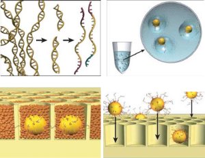
The figure goes in a clockwise direction. On the top left, DNA is fragmented into many pieces. Next in the upper right, the DNA is bound to tiny beads, one piece to a bead and the beads are isolated in little bubbles where the attached DNA is copied millions of times. This leaves each bead with millions of copies of a single piece of DNA. Importantly all these DNA are single stranded and looking for a matching strand. In the bottom right, the beads are deposited one to a well in a fiber optic slide. Then helper immobilization and enzyme beads fill in the wells in the bottom left. You can see some real images of this process in their next figure.

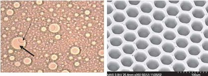
The left photo shows one of the beads (thin arrow) in a droplet (thick arrow). The bead is about 1/30 mm in diameter and the droplet about 1/10 of a mm. On the right is a electron micrograph of the wells on the fiber optic slide where beads are trapped. Each well is about 1/20 mm wide.

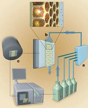
Once all this has been setup, they get to the real pyrosequencing part. With all the beads firmly nested in their separate wells, the sequencing machine takes turns flowing the A, T, C and G nucleotide building blocks of DNA over the wells. Because the DNA bound to the bead is single stranded, these new nucleotides begin building the second strand nucleotide by nucleotide. The trick to this technique (and where its name comes from) is that when a nucleotide is incorporated pyrophospate is released. This pyrophosphate is converted to ATP (a very common energy storage molecule) by enzymes on the helper beads. The ATP then fuels a bioluminescent luciferase enzyme (like in fireflies) to produce light. A 16 megapixel camera captures this light and the number of nucleotides incorporated can be estimated from the brightness. By cycling through T, A, C, and G around 40 times, the machine can count the number of bases incorporated in each step and get an average read length of about 110 bases. You can see that process in the following figure with (a) the nucleotides ready to flow over (b) the wells with their beads and produce light which is captured by (c) the camera and analyzed.

The authors were a little worried whether the shorter 110 base sequences would be useful. So they tried to sequence a bacteria, Mycoplasma genitalium. Although it’s sort of an easy target since this bacteria has a tiny 580,000 base genome, they did get an extremely thorough 40x coverage from a single run and were able to successfully assemble an accurate sequence of the genome.

The Rest of the Story

What they don’t mention in the paper is that one sequencer costs $500,000. Each run costs about $10,000 in chemicals and reagents (still cheaper than Sanger sequencing). Perhaps unsurprisingly at those prices, the 454 company responsible for this paper was later bought (for $150 million) by Roche, one of the largest pharmaceutical companies in the world.

Reminiscent of many gadgets, early adopters buying the sequencer from this paper got kind of screwed because 454 soon came out with a new improved model able to generate sequences twice as long. It looks like they’ll soon releasing an upgrade for the second model that should allow 2-4 times as many reads and again double the length (resulting in 8-16 times as many bases as this Nature paper).

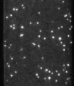
The paper is a little short of pictures direct from the sequencing process so here’s a couple from a recent run. First, here’s an example of a single flow (a T nucleotide [no visible difference from other nucleotides]) showing 13 lanes of a 16 lane slide (you can divide the slide into portions to share the run [and the cost]). You might notice a pattern in some of the lanes. That’s because lanes 1-4 and 9-12 were tests to see how much DNA per bead produced the best results with the lowest concentration on the left.

And here’s a close up of a single lane during a flow (a C this time). Each bright dot signals incorporation of a C nucleotides. Brighter dots mean there were several C’s in a row.

So a very cool technology. It’s pretty amazing that an entire bacterial genome (up to about 1.5 million bases [soon to be 6 million]) can be sequenced in one shot. Unfortunately, animals including humans have genomes of 2 billion or more bases so no one will be sequencing any individuals or endangered species without a few hundred thousand dollars to burn. But a little over ten years ago, you could get published in Science for sequencing the M. genitalium and here it was used as a simple test. It’ll be interesting to see where sequencing technology stands ten years from now.

References

Margulies, M., Egholm, M., Altman, W.E., Attiya, S., Bader, J.S., Bemben, L.A., Berka, J., Braverman, M.S., Chen, Y., Chen, Z., Dewell, S.B., Du, L., Fierro, J.M., Gomes, X.V., Godwin, B.C., He, W., Helgesen, S., Ho, C.H., Irzyk, G.P., Jando, S.C., Alenquer, M.L., Jarvie, T.P., Jirage, K.B., Kim, J., Knight, J.R., Lanza, J.R., Leamon, J.H., Lefkowitz, S.M., Lei, M., Li, J., Lohman, K.L., Lu, H., Makhijani, V.B., McDade, K.E., McKenna, M.P., Myers, E.W., Nickerson, E., Nobile, J.R., Plant, R., Puc, B.P., Ronan, M.T., Roth, G.T., Sarkis, G.J., Simons, J.F., Simpson, J.W., Srinivasan, M., Tartaro, K.R., Tomasz, A., Vogt, K.A., Volkmer, G.A., Wang, S.H., Wang, Y., Weiner, M.P., Yu, P., Begley, R.F., Rothberg, J.M. (2005). Genome sequencing in microfabricated high-density picolitre reactors. Nature DOI: 10.1038/nature03959